Bandpass Sampling: How to Digitise a 10.7 MHz IF FM Radio Signal with an ADC of 10 MHz Sampling Frequency?

What You Already Know: Nyquist Sampling

If you have studied Nyquist sampling, your instinct when you see a 10.7 MHz signal is to reach for an ADC running at at least 21.4 MHz. That instinct is correct for baseband signals — but it is wrong for bandpass signals, and understanding why opens up one of the most useful techniques in practical RF and communications engineering.

This article explains bandpass sampling from first principles, derives the conditions that make it work, walks through a concrete example using a 10.7 MHz intermediate frequency (IF) signal sampled by a 10 MHz ADC, and covers where the technique runs out of road.

The Nyquist–Shannon sampling theorem states that to perfectly reconstruct a signal, you must sample it at a rate at least twice its highest frequency component:

$f_s \ge 2f_{max}$

For a baseband signal — one that occupies frequencies from DC (0 Hz) up to some maximum frequency f_max — this is the rule you must follow. A 10 MHz audio or sensor signal genuinely requires a 20 MHz or faster ADC.

But here is the key insight that Nyquist is often misquoted as missing: the theorem actually says you need to sample at twice the bandwidth of the signal, not twice its centre frequency. For a baseband signal, bandwidth and maximum frequency are the same thing. For a bandpass signal, they are very different.

Bandpass Signals Are Different

A bandpass signal does not start at DC. It occupies a band of frequencies centred around some carrier or intermediate frequency. In communications and RF engineering, almost every signal of practical interest is a bandpass signal — AM, FM, Bluetooth, Wi-Fi, IF stages in superheterodyne receivers, and so on.

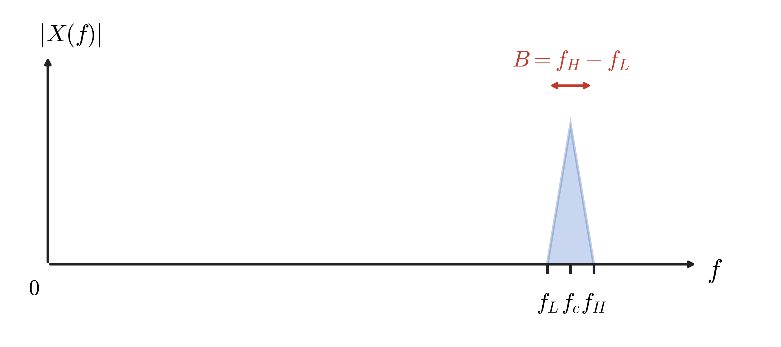
Bandpass signal spectrum showing bandwidth B much smaller than centre frequency f_c — Fig1 — Bandpass signal: bandwidth B is much smaller than centre frequency f_c

Bandpass Signal — the signal occupies a narrow band [f_L, f_H] centred on f_c. Because B << f_c — the bandwidth is much smaller than the centre frequency — you only need to sample at a rate F_s ≥ 2B, not twice f_c, to capture the signal without loss.

The 10.7 MHz IF signal used in FM radio receivers is a perfect example. After the RF front end mixes the received signal down from its broadcast frequency, it produces a signal centred at 10.7 MHz. This signal has a bandwidth of perhaps 200 kHz (for mono FM) — but its highest frequency component is about 10.8 MHz.

Applying Nyquist naively says you need a 21.6 MHz ADC. Bandpass sampling says you need a 400 kHz ADC — or any ADC running above 400 kHz that satisfies a specific set of conditions. A 10 MHz ADC is more than sufficient, as we will show.

The figure below makes this concrete. It takes exactly the case just described — a bandpass signal whose bandwidth is tiny compared to its centre frequency — and shows what happens when you actually sample it: the 10.7 MHz IF signal, sampled at just 10 MHz, doesn’t get destroyed by aliasing. Instead it reappears, fully intact, at 700 kHz. That’s the practical payoff of the bandwidth-not-centre-frequency rule above. The explanation right after the figure walks through why it lands exactly there, in terms of Nyquist zones and spectral inversion.

Bandpass sampling applied to a 10.7 MHz IF signal: continuous spectrum at ±10.7 MHz versus sampled spectrum replicas at Fs = 10 MHz, aliasing to ±700 kHz — Figure 2 — Bandpass signal sampling applied to a 10.7 MHz IF: (a) original continuous spectrum, B = 200 kHz; (b) sampled spectrum replicas at F_s = 10 MHz — the signal aliases to ±700 kHz.

Describing the figure

The top row (a) shows the original, continuous IF spectrum before sampling. Because the signal is real-valued, it has mirror-image energy at both +f_c and −f_c — here centred at 10.7 MHz, with an occupied bandwidth B of 200 kHz. Nothing unusual so far; this is just what a 10.7 MHz bandpass signal looks like on a spectrum analyzer.

The bottom row (b) shows what happens after that signal is sampled at F_s = 10 MHz. Sampling doesn’t just capture the signal — it stamps out a repeated copy of the entire spectrum at every multiple of F_s, spaced exactly F_s apart (shown by the two F_s double-arrows). The two original humps at ±f_c are still visible, but a new pair of images has now appeared much closer to DC, at −0.7 MHz and +0.7 MHz. Those two are the aliases: they exist precisely because 10.7 MHz and its repeated images (10.7 − 10 = 0.7, and −10.7 + 10 = −0.7) land inside the same low-frequency region. That ±700 kHz pair is the “down-shifted” copy of the original 10.7 MHz signal — it carries exactly the same information, just moved to a frequency the ADC’s baseband processing can work with directly.

Image Locations for an Undersampled Signal

$f_{image} = f_c + nF_s, \quad n = 0, \pm 1, \pm 2, \pm 3, \dots$

Nyquist Zones

A Nyquist zone is just a slice of the frequency axis wide. Each zone is exactly one “Nyquist bandwidth” further out than the last:

Zone 1:
Zone 2:
Zone 3:
Zone 4:
Zone k:

Nyquist zones 1 through 5 for a 10 MHz sampling rate, showing the real 10.7 MHz IF signal sitting in Zone 3 and aliasing down to 0.7 MHz in Zone 1 — Figure 3 — Nyquist zones 1–5 for F_s = 10 MHz. The real 10.7 MHz IF signal lands in Zone 3; sampling folds it down to 0.7 MHz in Zone 1. The asymmetric shape flips in Zones 2 and 4, showing the spectral inversion that even-numbered zones introduce.

Nyquist zones around a real 10.7 MHz signal sampled at 1 MHz, showing the signal landing in Zone 22 and aliasing down to 0.30 MHz in Zone 1, spectrally inverted — Figure 4 — Nyquist zones around a real 10.7 MHz signal, F_s = 1 MHz. The signal lands in Zone 22 (even); sampling folds it down to 0.30 MHz in Zone 1, spectrally inverted.

The Bandpass Sampling Theorem

When you sample a signal, you do not just capture it — you also create copies of its spectrum at every integer multiple of the sampling frequency. This is aliasing, and for baseband signals it is a problem to be avoided. For bandpass signals, it is a feature to be exploited.

The bandpass sampling theorem states that a bandpass signal with lowest frequency f_L, highest frequency f_H, and bandwidth B = f_H - f_L can be perfectly reconstructed from samples taken at rate F_s provided a suitable integer k exists such that:

$\dfrac{2f_H}{k} \le F_s \le \dfrac{2(f_H-B)}{k-1}$
and
$k \le \dfrac{f_H}{B}$

The key insight — Aliasing is usually an enemy. In bandpass sampling, you deliberately allow the signal to alias — but you choose the sampling rate so that the alias lands exactly where you want it in the baseband of the digital domain. The signal is still perfectly represented; it has just been frequency-shifted by the sampling process.

The integer k selects which alias, or which Nyquist zone, of the signal you are working with. For each valid k, there is a range of sampling frequencies that will place the aliased copy of the signal cleanly in baseband without overlapping anything else.

Where these conditions come from

Split the frequency axis into Nyquist zones, each of width F_s/2:

$\text{Zone } k = \left[(k-1)\dfrac{F_s}{2},\; k\dfrac{F_s}{2}\right], \qquad k = 1, 2, 3, \dots$

Sampling folds whichever zone your signal happens to sit in down into the base zone [0, F_s/2]. That folding is completely harmless — the signal is still fully recoverable — as long as the entire band [f_L, f_H] sits inside one single zone. If the band straddles a zone boundary, one half folds one way and the other half folds the opposite way, and the two halves land on top of each other in the digitised output. That kind of corruption cannot be undone afterwards.

So the whole derivation reduces to one requirement: pick a zone index k such that the band fits entirely inside zone k:

$f_H \le k\dfrac{F_s}{2} \qquad \text{and} \qquad (k-1)\dfrac{F_s}{2} \le f_L$

Rearranging each inequality for F_s gives the two halves of the boxed condition:

$\text{from } f_H \le k\dfrac{F_s}{2}: \qquad F_s \ge \dfrac{2f_H}{k}$

$\text{from } (k-1)\dfrac{F_s}{2} \le f_L: \qquad F_s \le \dfrac{2f_L}{k-1} = \dfrac{2(f_H-B)}{k-1}$

since f_L = f_H - B. Put together:

$\dfrac{2f_H}{k} \le F_s \le \dfrac{2(f_H-B)}{k-1}$

That window only exists at all if the lower bound doesn’t exceed the upper bound. Setting 2f_H/k ≤ 2(f_H-B)/(k-1) and solving for k:

Worked Example: 10.7 MHz IF Sampled at 10 MHz

FM radio receivers produce an intermediate frequency (IF) signal centred at 10.7 MHz. A typical wideband FM channel has a bandwidth of 200 kHz, so the signal occupies:

$f_L = 10.7\text{ MHz} - 100\text{ kHz} = 10.600\text{ MHz}$

$f_H = 10.7\text{ MHz} + 100\text{ kHz} = 10.800\text{ MHz}$

$B = f_H - f_L = 200\text{ kHz}$

$f_c = 10.7\text{ MHz} \quad \text{(centre / IF frequency)}$

Step 1 — Find the valid range of k

$k_{max} = \left\lfloor \dfrac{f_H}{B} \right\rfloor = \left\lfloor \dfrac{10.800}{0.200} \right\rfloor = \lfloor 54 \rfloor = 54$

So k can be any integer from 1 to 54.

Step 2 — Find which k values allow F_s = 10 MHz

For each candidate k, the valid sampling rate range is:

$\dfrac{2f_H}{k} \le F_s \le \dfrac{2f_L}{k-1} \qquad\Longrightarrow\qquad \dfrac{21.6}{k} \le 10 \le \dfrac{21.2}{k-1}$

Solving for k:

$\text{Left: } \dfrac{21.6}{k} \le 10 \;\Rightarrow\; k \ge 2.16 \;\Rightarrow\; k \ge 3$

$\text{Right: } 10 \le \dfrac{21.2}{k-1} \;\Rightarrow\; (k-1) \le 2.12 \;\Rightarrow\; k \le 3.12 \;\Rightarrow\; k \le 3$

$\therefore \;\; k = 3 \text{ is the only valid integer}$

Step 3 — Verify the sampling rate window

$\text{Lower bound: } \dfrac{2 \times 10.800}{3} = 7.200\text{ MHz}$

$\text{Upper bound: } \dfrac{2 \times 10.600}{2} = 10.600\text{ MHz}$

$\text{Valid range: } \;\; 7.200\text{ MHz} \le F_s \le 10.600\text{ MHz}$

Our ADC: F_s = 10 MHz ✓ — falls comfortably within the window.

Result

A 10 MHz ADC can perfectly digitise a 10.7 MHz IF signal with 200 kHz bandwidth. The alias of the signal (k = 3) lands at baseband after sampling, computed directly as 10.7 mod 10 = 0.7 MHz. The digitised signal appears centred at 700 kHz in the digital domain, ready for digital demodulation.

Practical Implementation Considerations

1. Anti-Alias Filter — More Critical Than Ever

In conventional Nyquist sampling, the anti-alias filter simply removes everything above f_s/2. In bandpass sampling it must do two things: pass the signal band you want (10.6–10.8 MHz) and reject everything else — especially other signals that might alias into the same baseband region. A bandpass filter centred at 10.7 MHz with tight skirts is essential before the ADC.

Critical warning — Any signal at a frequency that aliases to the same baseband location as your wanted signal will corrupt the digitised output irreversibly. The anti-alias filter must reject these interferers before sampling. This is the most common failure mode in bandpass sampling designs.

2. Sampling Rate Must Stay Inside the Valid Window

For our example the valid range was 7.2 MHz to 10.6 MHz. A 10 MHz ADC sits comfortably inside this window — but only 600 kHz away from the upper bound. If the ADC clock drifts, or if temperature causes the IF filter centre frequency to shift, the window could be violated. Design with margin — don’t sit right at the edge.

3. ADC Aperture Jitter

Because the signal being sampled is at 10.7 MHz (not 700 kHz), any jitter on the ADC sample clock causes phase noise proportional to the input frequency, not the alias frequency. The jitter-induced noise floor is:

$SNR_{jitter} \approx -20\log_{10}\left(2\pi f_{input}\, t_{jitter}\right)$

$\text{For } f_{input}=10.7\text{ MHz},\; t_{jitter}=1\text{ ps}: \quad SNR_{jitter} \approx 83\text{ dB}$

This is the ceiling on your dynamic range. A 12-bit ADC has a theoretical SNR of about 74 dB, so 1 ps jitter is fine. But at 10 ps jitter the ceiling drops to 63 dB and you are below 12-bit performance. Use a low-jitter clock source.

4. Digital Downconversion After Sampling

After sampling, your signal sits at 700 kHz in the digital domain. From here, standard digital downconversion applies: multiply by a digital local oscillator at 700 kHz to shift to baseband, then lowpass filter and decimate to your final sample rate. This is exactly what a software-defined radio (SDR) does in its digital backend.

5. Verify Your Alias Frequency

The alias frequency depends on the exact relationship between your signal and the sampling rate. For a signal at f_c sampled at f_s:

$f_{alias} = \left| f_c - \text{round}\!\left(\dfrac{f_c}{f_s}\right) \times f_s \right|$

$= |10.7\text{ MHz} - \text{round}(10.7/10)\times 10\text{ MHz}| = |10.7 - 1\times10| = 0.7\text{ MHz} = 700\text{ kHz}$

Limitations of Bandpass Sampling

Bandpass sampling isn’t free. It trades a lower ADC sample rate for tighter tolerances almost everywhere else in the signal chain, and it stops paying off once a few conditions aren’t met. Worth being clear-eyed about where it runs out of road.

The valid window shrinks as k grows

At k = 1 the window is unbounded above — that’s just ordinary Nyquist sampling, F_s ≥ 2f_H. As k rises, the window 2f_H/k ≤ F_s ≤ 2(f_H-B)/(k-1) narrows, exactly as the wedge diagram above shows. In our example (k = 3) the window was still a healthy 7.2–10.6 MHz. At higher k the usable slice can shrink to a few hundred kHz. A narrow window leaves little room for oscillator drift, temperature-driven filter shifts, or component tolerance — any of which can silently push you outside the window and corrupt the signal intermittently.

It only pays off for genuinely narrowband signals

The whole technique depends on B << f_c. As the fractional bandwidth B/f_c grows, k_max = ⌊f_H/B⌋ shrinks toward 1, and the valid windows collapse back toward plain Nyquist sampling. Wideband IF signals, or signals spread across multiple non-contiguous bands, gain little or nothing from undersampling.

ADC analog bandwidth and linearity still matter

The sample rate can be low, but the ADC’s analog front end — the track-and-hold circuit and input buffer — still has to faithfully acquire a signal at the real input frequency (10.7 MHz here, or higher in other designs). Datasheet SNR and ENOB numbers are usually specified at low input frequency; both typically degrade as the input climbs into higher Nyquist zones, even though the sample rate hasn’t changed. Check the SNR/SFDR-vs-input-frequency curve, not just the sample-rate spec.

Clock jitter requirements get harder, not easier

Undersampling doesn’t relax the clock budget. Jitter-limited SNR depends on the actual input frequency, not the alias frequency — and bandpass sampling is often used specifically to reach higher IF frequencies, where the jitter tolerance is tighter than it would be for an equivalent baseband design.

Anti-alias filtering gets harder as the window narrows

A wide window (low k) tolerates a fairly loose bandpass filter. A narrow window (high k) demands steep skirts close in frequency to the passband — which usually means higher order, higher Q, more expensive, and more group delay. There’s a practical ceiling on how large a k is worth using before the filter itself becomes the limiting factor.

No graceful degradation

The valid F_s window is a hard mathematical boundary, not a soft one. Stepping outside it doesn’t gently reduce SNR — it aliases an interferer directly on top of your wanted signal, and that corruption is unrecoverable after the fact. Real designs need deliberate guard-band margin, which eats further into an already-narrow window at high k.

Everything else in-band aliases too

Whatever the anti-alias filter fails to reject — thermal noise skirts, adjacent-channel interferers, harmonics from elsewhere on the board — lands on top of the wanted signal, indistinguishably, once sampled. Bandpass sampling does not reduce the total noise reaching the ADC; it relies entirely on the analog filtering having already done that job, since there’s no way to undo it digitally afterward.

Summary

Bandpass sampling is one of those techniques that seems almost too good to be true when you first encounter it. A 10 MHz ADC digitising a 10.7 MHz signal — surely that violates Nyquist? It does not, because Nyquist’s requirement is on bandwidth, not on centre frequency. The 200 kHz wide IF signal has a bandwidth that a 10 MHz ADC can handle with ease. But the technique only works within a well-defined window, and that window narrows the harder you push it.

→Nyquist requires 2× bandwidth, not 2× centre frequency. For bandpass signals, bandwidth ≪ centre frequency — so the required sample rate is far lower than intuition suggests.

→The valid F_s window comes from fitting the band inside one Nyquist zone. That single geometric requirement is the whole derivation behind both boxed conditions.

→Aliasing is deliberate here. The k = 3 alias of the 10.7 MHz signal lands at 700 kHz after 10 MHz sampling.

→The window narrows as k grows, and it isn’t free. Tighter windows demand tighter clocks, tighter filters, and leave no margin for drift.

→Anti-alias filtering is critical. Any interferer that aliases to the same location as your signal corrupts the output permanently.

→Aperture jitter is referenced to the input frequency, not the alias frequency — undersampling doesn’t relax the clock budget.

→Follow with digital downconversion. After sampling, multiply by a 700 kHz NCO and lowpass filter to recover the baseband signal for demodulation.